What do we mean when we say “Bayesian inference”? More specifically, what does Bayesian inference mean for my machine learning or data modelling problem? In this blogpost I will introduce Bayesian inference and explain how it is a machine learning paradigm. More importantly I will attempt to intuitively bridge the gap between Bayesian inference as a theoretical framework and Bayesian inference as a machine learning approach.

The Real World: Data and Modelling

Let’s begin with the problem which we’re trying to solve in the first place: we have some acquired data and we would like to predict future instances. Using the same starting point as my post on neural ODE’s, we can formalise this setting as follows:

We have \(N\) observations of \(x, y\): \(\mathscr{D} = \big\{(x_1, y_1), (x_2, y_2), …, (x_N, y_N)\big\}\). \(\mathscr{X}\) is the input domain and \(\mathscr{Y}\) is the output domain.
Given a new input, \(x^{*}\), we would like to predict the unknown output: \(y^{*}\).
We assume that there is some function which maps the input and output domains: \(f:\mathscr{X} \to \mathscr{Y}\).

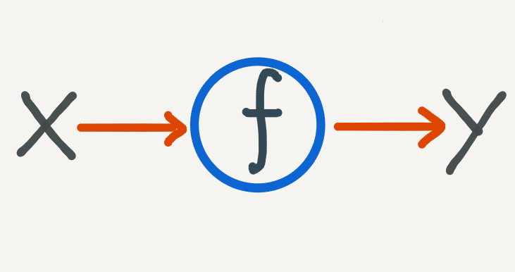
We model the problem as trying to find a function mapping from \(\mathscr{X}\) to \(\mathscr{Y}\).

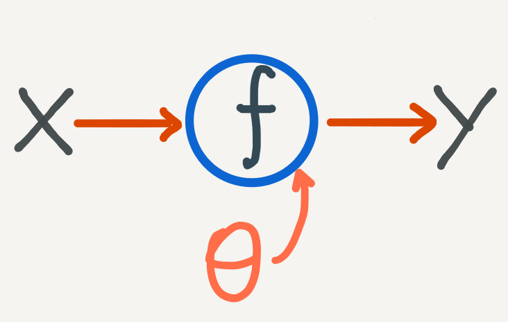
The machine learning approach is to choose a flexible class of functions, typically neural networks, which are described by parameters \(\theta\). We use a learning algorithm, such as stochastic gradient descent, to optimize the parameters \(\theta\) such that the function \(f\) is a good fit for the data. What we mean by a “good fit” is codified by a cost function which is minimized during the learning procedure. Traditionally this cost function measures the degree to which the data fits the model well. If not, then adjust the parameters of the model and measure again until the cost is sufficiently low.

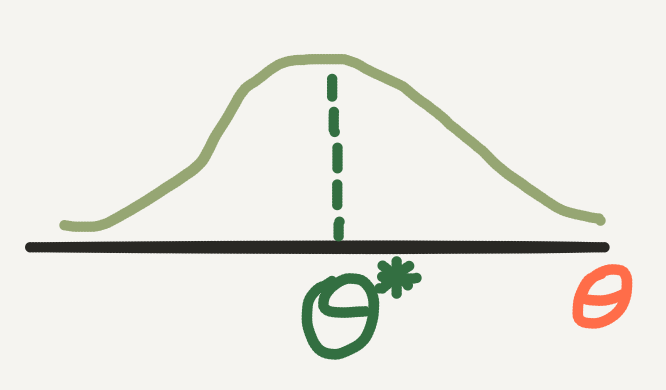
We then make new predictions using the optimal parameter \(\theta^{*}\). One shortcoming of this approach is that once we have found the optimal \(\theta^{*}\), the prediction process is completely deterministic. This is a problem if we require uncertainty in our predictions:

How certain are we that patient \(\mathscr{x}\) will have outcome \(\mathscr{y}\)?
How certain are we that image \(\mathscr{x}\) can be classified as \(\mathscr{y}\)?
How certain are we that measurement \(\mathscr{x}\) will yield signal \(\mathscr{y}\)?

In general uncertainty is desirable if the variance in the data is large. The learning algorithm finds \(\theta^{*}\) which works for most of the data points which we’ve seen so far. How reliable will \(\theta^{*}\) be, when \(\mathscr{x}\) is an outlier - when it is not like most datapoints?

Uncertainty is also desirable when we don’t have a large number of samples. In this case, if the variance is large between each sample, then we may not have enough evidence to support any one particular value of \(\theta\). Instead we would like a way of making predictions which accounts for our uncertainty on the value of the parameter \(\theta\) itself.

This is precisely what we will try to achieve with Bayesian inference.

An old favourite: Bayes’ Theorem

As the name implies, Bayesian inference has a lot to do with Bayes’ Theorem. In fact, Bayes’ Theorem will form the bridge between the uncertainty in our data and the uncertainty in our predictions. You may already be familiar with Bayes’ Theorem (which I also covered in my post on conditional probability), but as a recap here is what we mean by Bayes’ Theorem:

Let \(A\) and \(B\) be random variables\(^{*}\) with probability measure \(\mathbb{P}\), such that \(\mathbb{P}(A) \neq 0\), then \[ \mathbb{P}(B|A) = \frac{ \mathbb{P}(A | B)\mathbb{P}(B) }{ \mathbb{P}(A) }. \]

\(\mathbb{P}(B)\) is known as the prior probability of \(B\) - it is what we know (assume) about \(B\) before we consider the effects \(A\).

\(\mathbb{P}(A)\) is known as the evidence of \(A\) - it is everything we know about \(A\).

\(\mathbb{P}(A | B)\) is known as the likelihood of \(A\), given \(B\) - it is an estimate of how likely the \(A\) that we observed is, given possible values of \(B\).

\(\mathbb{P}(B | A)\) is known as the posterior probability of \(B\), given \(A\) - it is the conditional probability of \(B\) after we have obtained evidence of \(A\).

Bayes’ Theorem is useful when it is difficult to calculate the posterior of \(B\) directly. We use Bayes’ Theorem when we have obtained data on \(A\) and we can measure the likelihood and prior with greater ease.

* for more detail on random variables and probability measures, see my introductory post on probability.

Bayes’ Theorem Meets the Real World

Let’s go back to the fundamental modelling problem. We have a parametric function, described by \(\theta\), and we want to choose the right \(\theta\) so that our function describes the data well. We also want to compute our uncertainty over \(\theta\) so that we can make predictions with confidence, and know when this uncertainty is high.

But what does it mean to include uncertainty into our modelling of \(f\) and \(\theta\)?

This means precisely to use probabilities - the mathematical language of uncertainty - and in particular it means to use probability distributions. Instead of optimizing for a single value of \(\theta\), we can treat \(\theta\) as a random variable which has highest probability at the optimal value.

But how do we ensure that the probability distribution over \(\theta\) has highest probability at the optimal value?

We do this by using Bayes’ Theorem. In particular we can start with a best guess at what this distribution may be and call it our prior distribution

\[ P(\; \theta \;)^{*}. \]

How do we know what a good prior distribution is?

This is a difficult question but in theory our choice on the prior doesn’t matter if are able to obtain enough data. In practice the choice of prior will affect the posterior and it helps to encode (and test!) our assumptions on \(\theta\). For example use a discrete probability distribution if \(\theta\) is discrete, or a positive distribution if \(\theta\) must be non-negative.

What’s important in Bayesian inference is that whatever choice of prior we choose, the additional data which we obtain will alter the shape of prior to inform our target posterior distribution. Going back to Bayes’ Theorem we can incorporate the data \(\mathscr{D}\) into the formula using the likelihood

\[ P(\; \mathscr{D} \;|\; \theta \;). \]

It is through the likelihood that we encode the optimality of \(\theta\) into the posterior, which is defined by the degree to which \(\theta\) is a good fit for the data. Strictly speaking the likelihood is a function of \(\theta\) - we assume the data has been observed and is fixed. With this point of view the likelihood can be interpreted as the likelihood of the observed data occurring, given the possible values of \(\theta\). A higher likelihood indicates a better value of \(\theta\).

In fact many machine learning loss functions are derived from the likelihood, usually in the form of the negative log-likelihood (applying the log transformation to the likelihood helps for numerical stability purposes, especially over a large dataset).

The likelihood function does not need to strictly be a probability distribution.

Now we can use Bayes’ Theorem to write down a formula for the posterior distribution of \(\theta\):

\[ P(\; \theta \;|\; \mathscr{D} \;) = \frac{ P(\; \mathscr{D} \;|\; \theta \;)P(\; \theta \;) }{ P(\; \mathscr{D} \;)}. \]

The posterior distribution takes into account our uncertainty over \(\theta\) (incorporated in the prior distribution), adjusted by the actual data that we observed (incorporated in the likelihood, and also the evidence of the data). The combination of the likelihood with the prior makes the posterior distribution suitable for estimating optimal values of \(\theta\) with the added measure of uncertainty.

How does this posterior distribution help us?

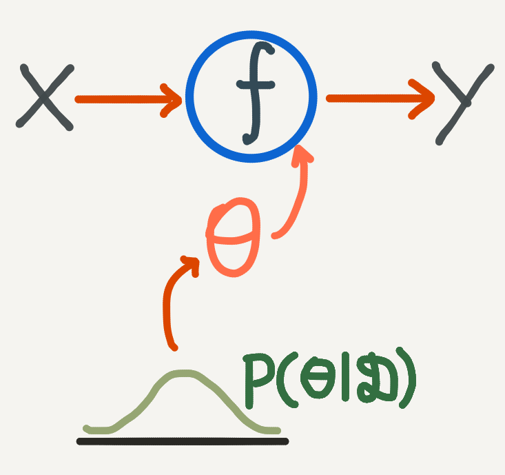
Instead of calculating a single estimate of the optimal \(\theta\) we look for a (posterior) distribution on \(\theta\). From this distribution we can calculate a sample mean for \(\theta\) and report our confidence over a credible interval - say the middle 95% of the distribution.

Going back to the original function estimation problem, this means that when we calculate predictions for \(\mathscr{y}\), we first estimate \(\theta\) from the posterior so that our predictions become conditional on \(\theta\):

But it turns out that calculating this posterior can be hard with a capital H. For two reasons:

The likelihood function is often highly nonlinear and must include every sample from the training dataset. In addition the complexity of the likelihood increases with the dimension of the data.
The evidence, \(P(\; \mathscr{D} \;)\), can be extremely hard to compute. It requires knowing how much probability to assign to every possible value which the data can take. In an uncertain world this is practically impossible.

The algorithmic insight is to use what’s called approximate inference. Instead of calculating the posterior directly, we will try to approximate it.

*Note: that whereas before I used blackboard bold \(\mathbb{P}\) to denote the probability measure for individual probabilities, here I am using plain \(P\) to denote a probability distribution function. These are subtly different things conceptually and the change in notation is a pedantic way of expressing that. In short the probability distribution function is a function which describes all of the probabilities of a random variable over its domain.

Approximate Inference

Broadly speaking there are three main types of approximate inference algorithms, with the first two being the most popular. Briefly, they are:

Monte Carlo Sampling: this is a broad class of algorithms which approximates a target distribution by computing samples. In Bayesian inference we use a special type of Monte Carlo sampling algorithm known as Markov Chain Monte Carlo (MCMC) which iteratively computes samples using only information from the previous sample and the target distribution we are trying to approximate: \[ \theta_{t} \leftarrow \theta_{t-1}, \ \theta_{t} \sim P(\; \theta \;|\; \mathscr{D} \;). \] With Monte Carlo algorithms, we do not try to explicitly compute the distribution, but rather try to compute candidate samples for \(\theta\) until eventually most samples are close to the optimal value of \(\theta\).
Variational\(^{*}\) Inference: here we attempt to approximate the posterior distribution itself. We do this in much the same way that we use machine learning to approximate a function: choose a flexible function \(q\) parametrised by \(\phi\) and optimise \(\phi\) so that \[ q(\theta) \approx P(\; \theta \;|\; \mathscr{D} \;). \]
Expectation Propagation: again we approximate the posterior with a tractable function \(q\), except we specifically choose this function to be factorisable into a product of distributions which are conditional on each other. We then use message passing algorithms to iteratively update the factors of \(q\) until it is a good fit for the posterior.

While I won’t go into more detail into each of these algorithms - they are entire blogposts (and more!) unto themselves - I will try and unravel the basic fundamentals of approximate inference for the remainder of this blopost.

\(^{*}\)The name variational inference comes from variational calculus which is the calculus of finding functions by varying their parameters. The function \(q\) is sometimes known as the guide.

A Chicken and Egg problem

You may have noticed that approximate inference has a chicken and egg problem. We want to approximate the posterior by drawing samples, but how can we draw samples from the posterior if we can’t compute it directly? Or we want to approximate the posterior with some parametrised guide distribution, but how do we know that it is a good match for the posterior without evaluating the posterior directly?

We get around this as follows:

The denominator in Bayes’ Theorem is a normalization constant. If we ignore this constant (a constant function really), then the posterior distribution is proportional to the product of the likelihood and the prior (both of which are computable to us), which we write as follows: \[ P(\; \theta \;|\; \mathscr{D} \;) \propto P(\; \mathscr{D} \;|\; \theta \;)P(\; \theta \;).
\]
Furthermore in approximate inference we are more interested in the argmax of the posterior distribution - which \(\theta\) has maximum probability? - rather than the probability on \(\theta\) itself. Thus we can exploit the property of optimization where if \(g\) is our objective function and \(C\) is a constant then: \[ argmax\{\; g \;\} = argmax\{\; \frac{1}{C}g \;\}. \]

In the case of MCMC specifically, we use an algorithm which explicitly does not require knowing \(P(\; \mathscr{D} \;)\) in order to update samples of \(\theta\), doing so until we start sampling the \(\theta\) with maximum probability.
Once we have the posterior up to a normalization constant, we simply need to normalize the posterior to turn it into a probability distribution.

Unravelling the graph

We can express the cyclic nature of Bayesian inference graphically in the following way:

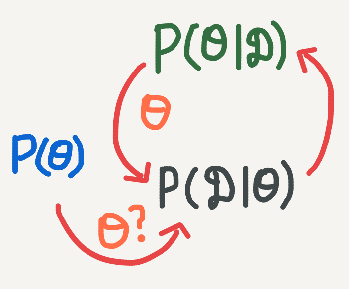
Start with a prior distribution on \(\theta\), which we can use to sample \(\theta\).

What is the likelihood of \(\theta\), given the data?

We get the posterior probability of \(\theta\), which we can use to sample a better estimate of\(\theta\).

But we can still test the likelihood of this \(\theta\)…

Now we can see what we are trying to do with Bayesian inference a bit better. Start with a prior and likelihood (going forwards on the graph), and then go backwards to calculate a suitable posterior. When we can’t calculate this posterior exactly (feasible for only the simplest of models), then we resort to approximate inference. Approximate inference works by iteratively updating the posterior (forwards) and then checking to see if the samples for \(\theta\) are good (backwards). In general approximate inference algorithms work as follows:

Given a prior distribution and likelihood function:

Choose an initial starting point for \(\theta\).
Use the likelihood function and prior to estimate a posterior (or posterior sample) from the current value of \(\theta\).
Suitably update the posterior based on how good (or bad) a fit we have so far.
Sample a new \(\theta\) value from the current posterior.
Repeat steps 2-4 until we get a suitable fit for the posterior.

Note: For variational inference we instead update the parameter \(\phi\) to obtain a good functional approximation of the posterior distribution, and from this approximation we will sample \(\theta\).

Going back to the graph, we are essentially unrolling the cyclic relationship between the posterior estimate and the sampling of \(\theta\) into a successive sequence of algorithm iterations:

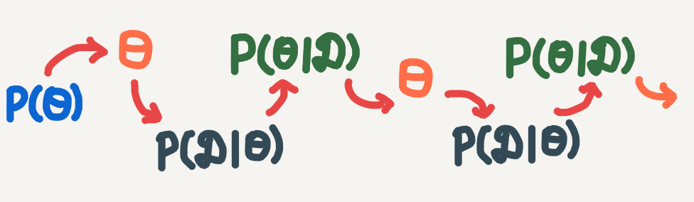
Start with an initial value for \(\theta\). Successively update the posterior and then sample a new estimate of \(\theta\).

The exact details of steps 2-4 and when we determine to terminate the algorithm will depend on the choice of algorithm used. Although these algorithms are beyond the scope of this introduction to approximate inference, I intend on covering them in future posts.

Tying it back together

What we have seen so far is that when we want to express uncertainty over the modelling parameters in a machine learning problem, we can use Bayes’ Theorem to help us. Specifically

When we have a dataset \(\mathscr{D} = \big\{(x_1, y_1), (x_2, y_2), …, (x_N, y_N)\big\}\),
And a model, \(f: \mathscr{X} \to \mathscr{Y}\), with parameters \(\theta\),
Then we can use Bayes’ Theorem to describe a posterior distribution over the modelling parameters \(\theta\), by specifying a prior distribution and a likelihood function so that: \[ P(\; \theta \;|\; \mathscr{D} \;) \propto P(\; \mathscr{D} \;|\; \theta \;)P(\; \theta \;). \]

Once we have this posterior distribution, we can make a prediction \(y^{*}\) at a new point \(x^{*}\), using the so-called predictive distribution - the probability distribution over \(y^{*}\) given \(x^{*}\) and our uncertainty over the parameters \(\theta\):

\[ P(\; y^{*} \;| x^{*}; \mathscr{D} \;) = \int_{\theta} P(\; y^{*} \;| x^{*}, \theta \;)P(\; \theta \;|\; \mathscr{D} \;)d\theta. \]

In practice we approximate \(P(\; y^{*} \;|\; x^{*}, \theta \;)\) by the function \(f\) and we can use the posterior distribution to compute samples \(\big\{ \theta_1, \theta_2, … \theta_M \big\}\). Then we can calculate a sample mean for \(y^{*}\) using a Monte Carlo estimate:

\[ y^{*} \approx \; \widehat{y} \; = \; \frac{1}{M}\sum_{s=1}^{M}f(x^{*}; \theta_s). \]

To measure the uncertainty of our prediction we can calculate a sample variance:

\[ Var(y^{*}) \approx \frac{1}{M}\sum_{s=1}^{M}\big( f(x^{*}; \theta_s) - \widehat{y} \big)^{2}. \]

Bayesian Inference is a Modelling Paradigm

In traditional machine learning we specify a model and try and find the parameters of the model which best fit the data. The cost function which we use, typically the likelihood, gives us a measure of how well the parameters fit the data.

Bayesian inference instead seeks to find the most probable parameters, given the data. By seeking most probable, we imbue the model with predictive uncertainty. In Bayesian inference we model a posterior distribution over the parameters.

Bayesian Inference is an Optimization Paradigm

In the traditional machine learning approach we can only find a single point estimate of the optimal parameter \(\theta^{*}\). This is known as a maximum likelihood estimate (MLE) and can be interpreted as follows: if true, we would likely observe the data which we have under this model.

In the Bayesian inference approach, we use the likelihood to reshape the prior distribution into a posterior distribution which places highest probability over the optimal \(\theta\). This \(\theta\) is sometimes known as the maximum a posteriori estimate (MAP), and can be interpreted as the parameter which is a best fit for the data, given our uncertainty.

Take note that when using the predictive distribution above we are not explicitly using the MAP estimate for \(\theta\) but rather taking many samples of \(\theta\). Of course if our uncertainty over \(\theta\) is not too large, than most of the \(\theta\) samples will be close to the MAP estimate.

In the algorithmic approach, our aim is to optimize \(\theta\) based on the data. Except now we can optimize \(\theta\) according to the posterior distribution.

Bayesian Inference is a Machine Learning Paradigm

In modern machine learning, Bayesian inference gives us a framework by which we can resolve the desire for an accurate algorithm with a measure of uncertainty. Using approximate inference we can scale Bayesian inference to large datasets and models with high dimensional parameters, such as neural networks.

Really this whole post has been about how we can rethink machine learning using Bayes’ Theorem, and that ultimately, is what Bayesian inference is.

Bonus: A Little Bit of Information Theory

In a way we can think of Bayesian inference (and machine learning in general) as an exercise in compression. We don’t have access to all the data in the world for our problem. Instead we use the data which we have to optimize the parameters \(\theta\) of a function which we hope can describe the relationship between \(\mathscr{X}\) and \(\mathscr{Y}\). In general the dimensionality of \(\theta\) is much lower than the data, so really we are compressing all the information in our dataset into the parameter \(\theta\).

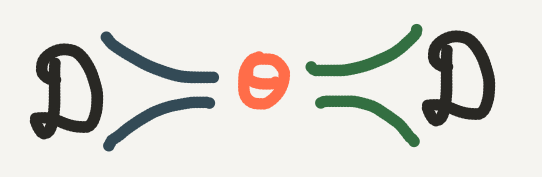
When we go in the forward direction of Bayesian inference, we are finding the \(\theta\) which most likely describes the data. In other words, the likelihood helps us to encode the data into \(\theta\). When we go in the backward direction (posterior inference), we sample many values of \(\theta\) to account for our uncertainty. If our posterior distribution is good, then we will almost always sample the optimal value of \(\theta\) such that such that we should be able to recover original dataset. In other worlds the posterior helps us to decode the input to our target values.

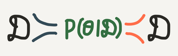
Photo by Dattatreya Patra on Unsplash

← Previous Post