This is the second in a series of blogposts which I am writing about probability. In this post I introduce the fundamental concept of conditional probability, which allows us to include additional information into our probability calculations. The ideas behind conditional probability lead naturally to the most important idea in probability theory, known as Bayes Theorem. As with the first post, which you can read here, the approach is to explain conditional probability using mathematical ideas from measure theory. Again, as with the first post, this post is meant to be accesible to anyone, regardless of whether you’ve studied maths or not.
A Game of Dice
In my last post I discussed probability as a way of the measuring the uncertainty of an event. We thought of probability as assigning a weight to the chance that an event has a particular outcome, which we measured relative to other possible outcomes. We defined an event space, which we called \(\Omega\). On this space of events we defined a random variable, \(X\), as a function which maps each event to our observed outcomes, encoded as numbers on the real line, \(\mathbb{R}\):
\[ X:\Omega \to \mathbb{R}. \]
The probability of an outcome is then the size of the number of possible events which are mapped to that outcome, relative to the size of the whole event space:
\[ \mathbb{P}:\mathscr{F} \to [0,1]. \]
We called the set of possible events the preimage of the random variable. If \(B\) is an outcome, then the preimage of \(B\) is \(X^{-1}(B)\) and the probability of \(B\) is the relative size of the preimage, given by \(\mathbb{P} \big((X^{-1}(B)\big)\).
For instance, in the dice example from the last post where we considered the experiment of rolling two die and adding the numbers, if we observe an outcome \(9\), then there were four possible events which could add up to 9, namely \((3,6)\), \((4,5)\), \((5,4)\) and (\(6,3)\). We called this set \(A\). Since there are \(36\) possible outcomes in \(\Omega\), we can then measure the probability of getting a \(9\) by the relative size of \(A\) with respect to \(\Omega\). If \(X\) is the random variable representing our experiment, then \(A\) is the preimage of the observation \(X = 9\), and the probability of A is
\[ \mathbb{P}(A) = \frac{4}{36} = \frac{1}{9}. \]
Thinking About the Past
However, what if we were able to incorporate information about events that have happened before? For example, suppose that instead of rolling the two die at once, we roll them one at a time. In this case, depending on the outcome of the first roll, the probability of getting a \(9\) will be different. To see how, let’s consider an example where our first roll is a \(3\). In the first scenario there was a total of 36 possibile configurations before any roll was made. However, now that we’ve observed one of the die as a \(3\), the total number of configurations is diminished,namely the set:
\[ B = \big\{(3,1), (3,2), (3,3), (3,4), (3,5), (3,6) \big\}. \]
In this case there is only one possible event leading to an outcome of \(9\): the event that we get a \(6\) on the second roll. How do we calculate the probability of \(9\) now? By the end of this blogpost we’ll see that calculating the total uncertainty will require a fundamental and important result in probability theory, known as Bayes’ Theorem. We’ll work our way towards that point, but for now we’ll start with the simplest scenario.
Using What We Already Know
We’ve reduced the problem to the event that we have already rolled a \(3\), so all of our uncertaintly only lies with the second roll. In this case we’ve seen that there are only \(6\) possible events in total with only one of them leading to a \(9\). Using the same logic from the previous post, the probability of rolling a \(9\), given that we have already rolled a \(3\) is:
\[ \mathbb{P}(\text{observe a }9 | \text{rolled a }3) = \frac{1}{6}. \]
The first thing to notice is that this probability is higher than the totally uncertain scenario, where \(\mathbb{P}(A) = 1/9\). This makes sense since rolling a \(3\) greatly increases our chances of getting a \(9\), even though there is only one valid configuration out of \(6\). To understand this better, suppose that we do not roll a \(\ 3\) on the first roll, then our space of possible events, which we’ll call \(\Theta\) (capital Greek letter “theta”) has \(30\) possible configurations. On this space there are \(3\) possible configurations leading to a 9, namely \((4, 5), (5, 4)\) and \((6, 3)\). So the probability of getting a \(9\) given that we do not roll a three on the first roll is:
\[ \mathbb{P}(\text{observe a }9 | \text{have not rolled a }3) = \frac{3}{30} = \frac{1}{10}, \]
which is less than the totally uncertain scenario, and even smaller than the scenario where we roll a \(3\) on the first throw. Clearly rolling a \(3\) on the first roll increases our chances of getting a \(9\).
In fact, it is more general than that. Any roll that increases our chances of landing in \(A\), which is after all the preimage of \(X = 9\), will increase our chances. This fundamental idea can be explained graphically.
The Shape of Probability
Let’s go back to an earlier statement where I said that the probability of an outcome \(B\) is given by the relative size of it’s preimage:
\[ \mathbb{P}(B) = \frac{size\big(X^{-1}(B)\big)}{size(\Omega)}. \]
Let’s unpack what this means graphically. We can visualise the events in \(\Omega\) as shaded regions - for example the set \(X^{-1}(B)\), which for simplicity we simply label as \(B\), is shown below:
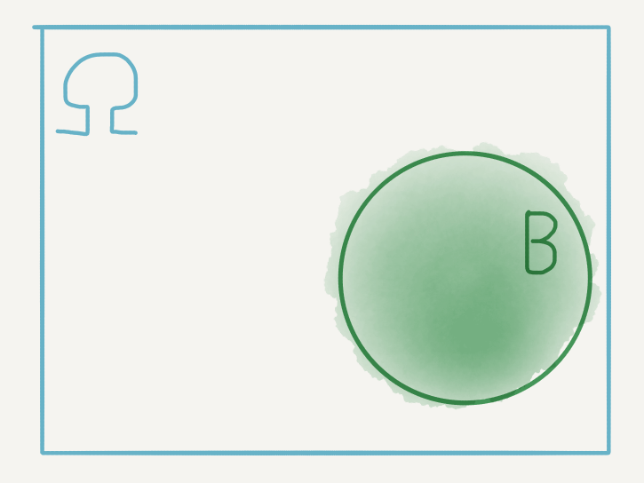
While these visualisations are just a heuristic and are too imprecise for measuring probabilities, they are helpful for visualising how different events interact, and hence how their probabilities may interact.
For example, if \(A\) is the event our rolls add up to \(9\), we can include that in our diagram and it is now clear that this event intersects \(B\) at exactly one point: the pair \((3, 6)\).
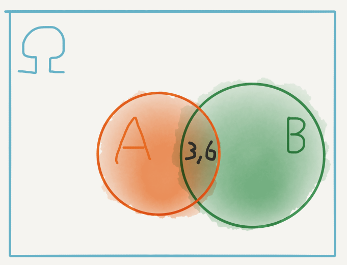
This was the one configuration leading to \(9\), with a \(3\) on the first roll. However, since this a point in \(\Omega\), why don’t we measure it’s probability as \(\mathbb{P}\big((3,6)\big)= 1/36\)? That would depend on what we were looking for. In particular we were interested in the probability of \(9\), given that we have already rolled a \(3\). If we have already rolled a \(3\), then we are no longer in the whole space \(\Omega\).
Configurations such as \((2, 4)\), \((1, 5)\) and \((4, 1)\) are no longer available to us, so clearly we have to redefine our space of interest.
Revaluating Size
To see how to do so, let’s go back to the diagram of \(A\) and \(B\). If we have already rolled a \(3\), the possible configurations available to us have shrunk from the whole of \(\Omega\) to just the set \(B\)! This shrinking action also excludes some of the configurations in \(A\), all except for \((3, 6)\), which is in the intersection of \(A\) and \(B\). We can think of this visually as:
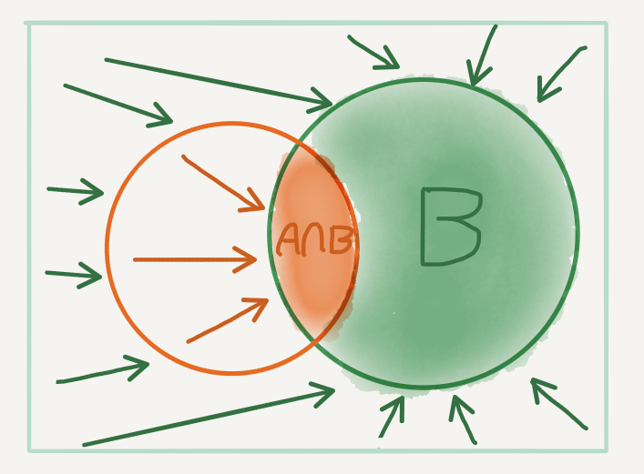
Now, when we take the probability of \(9\), given that we have rolled a \(3\), we have to revaluate how we measure size in context of what is now possible. The preimage of \(9\) is now just the intersection. Since the event \(B\) is assumed to have already happened (as visualised by the shrinking of the event space to \(B\)), we measure the size of the preimage relative to \(B\), so that
\[\begin{align} \mathbb{P}(\text{observe a }9 | \text{rolled a }3) & = \mathbb{P}(A | B) \\ & \\ & = \dfrac{size(A\cap B)}{size(B)} \\ & \\ & = \dfrac{1}{6}. \end{align}\]
Conditional Probability
What have just seen is known as the condtional probability of an event. It is the probability of the event \(A\), conditional on the event \(B\). By thinking of conditioning as a restriction on the size of the event space, we can measure the conditional probability of \(A\) given \(B\) as
\[ \mathbb{P}(A| B) = \frac{size(A\cap B)}{size(B)}. \]
We can make this even more intuitive by remembering that the probability of any event is given by the size of that event relative to the whole set, namely:
\[ \mathbb{P}(B) = \frac{size(B)}{size(\Omega)}. \]
A slight hand rearrangement gives:
\[ size(B) = size(\Omega)\mathbb{P}(B), \]
which we can do since \(size(\Omega)\) is always positive. We can get a similar formula for the set \(A\cap B\). Plugging both formulas back into our expression for the conditional probability gives
\[ \mathbb{P}(A| B) = \frac{size(\Omega)\mathbb{P}(A\cap B)}{size(\Omega)\mathbb{P}(B)}, \]
which simplifies to
\[ \mathbb{P}(A| B) = \frac{\mathbb{P}(A\cap B)}{\mathbb{P}(B)}. \]
Tying Back to Intuition
Intuitively this says that the probability of \(A\) given \(B\) is the probability of \(A\) and \(B\) divided by the probability of just \(B\). By deriving this formula in the example, we understand this division as the shrinking of the event space. Mathematically this shrinking action is referred to as the projection of the event space onto the conditioning space.
Immediately we know from elementary mathematics that the probability of \(B\) cannot be zero to avoid a division error. Indeed this reinforces our intution since we cannot condition on an impossible event!
Finally we can view the intersection as a restriction of our event of interest to the conditioning event. Indeed, the intersection of \(A\) and \(B\) can be thought of as the projection of the set \(A\) onto the set \(B\), which is the conditioning space.
All in all, we can think of conditional probability as probability which is projected onto some (smaller) conditioning space.
Bayes’ Theorem: The Fundamental Property of Probability
It turns out that the intersection is symmetric: the projection of \(A\) onto \(B\) is identical to the projection of \(B\) onto \(A\). Indeed the diagrams from earlier reinforce this.
Based on the same procedure we could have just as easily derived the conditional probability
\[ \mathbb{P}(B| A) = \frac{\mathbb{P}(A\cap B)}{\mathbb{P}(A)}. \]
Once again, since \(\mathbb{P}(A)\) is positive and cannot be zero, we can use a mathematical slight of hand to derive an expression for the probability of the intersection:
\[ \mathbb{P}(A\cap B) = \mathbb{P}(B| A)\mathbb{P}(A). \]
This says that the probability of \(A\) and \(B\) is the conditional probability of \(B\) given \(A\) times the probability of just \(A\).
Intuitively if we take the conditional probability of \(B\) given that \(A\) has already happened, and we factor in the probability of \(A\), we must be left with the probability of both.
But we know from earlier that if we have the probability of the intersection, we can project the conditioning space of \(B\) to calculate the inverse probability: the conditional probability of \(A\) given \(B\), which is given by:
\[\begin{align} \mathbb{P}(A | B) & = \dfrac{\mathbb{P}(A\cap B)}{\mathbb{P}(B)} \\ & \\ & = \dfrac{\mathbb{P}(B | A)\mathbb{P}(A)}{\mathbb{P}(B)}. \end{align}\]
This final result is known as Bayes’ Theorem.
In this formulation, if \(A\) is our event of interest and \(B\) is the conditioning event, then the quantity
\[ \mathbb{P}(A \vert B) \]
is known as the posterior probability of \(A\) given \(B\).
The quantity
\[ \mathbb{P}(B \vert A) \]
is known as the likelihood of \(A\) given \(B\).
Finally the quantity
\[ \mathbb{P}(A) \]
is simply known as the prior probability of \(A\).
Intuitively the prior of \(A\) is the raw probability of \(A\) before any other event is taken into consideration. The likelihood, although taken as a conditional probability of \(B\), can be thought of as a measure of how likely it is that \(A\) depends on \(B\). To understand why, recall that we derived the likelihood’s place in the formula by considering the symmetry of the intersection. Finally the posterior is the final probability of \(A\) after conditioning on \(\ B\).
The Importance of Bayes’ Theorem
Fundamentally, Bayes’ Theorem gives us a way of measuring conditional probability by taking into consideration our total uncertainty. This is the point I promised to get earlier this post. In the example, instead of considering each roll one at a time, then enumerating how the total event space changes after the first roll lands on a \(3\) we can measure \(\mathbb{P}(\text{observe a }9 \vert \text{rolled a }3)\) directly by considering all of the quantities in Bayes’ Theorem.
I’ll leave this as an exercise but by thinking carefully about the likelihood (hint: recall how we derived the likelihood using the symmetry of the intersection), you can calculate the posterior and see that it yields the same result.
Although it is not obvious from the elementary example which I used to derive conditional probability using measure theoretic intuition, there are situations where computing likelihoods is much easier than directly measuring the posterior of interest. This post was intended as an introduction to conditional probability, so I will not go into the details here. However, for those interested I suggest reading Chapter 3 of the late David MacKay’s book Information Theory, Inference and Learning Algorithms, which is available for free here.
Although ITILA (as it is abbreviated to) has been superseded by more modern machine learning textbooks (which, considering the pace of research in machine learning, don’t have long either before they are out of date), it still remains a fundamental reference for learning algorithms, especially from a probabilistic point of view.
What About Casuality?
There is a natural tendency to think of conditional probability as specifying a causal relationship. If we condition \(A\) on \(B\), does this mean that \(B\) causes \(A\). In general this is not the case and it is dangerous to fall into this trap. Indeed, in the derivation I argued that the conditioning action is somewhat symmetric in the sense that if we can condition on \(B\), then we can also condition on \(A\). In most cases this is true. In fact Bayes’ Theorem demands that we think of conditional probabilities (the posterior) as depending on their conditional inverse (the likelihood).
Causality is one of the least well understood concepts in statistics. It requires that we rethink how statistical relationships are modelled. In the future, depending on how well I can understand the basic ideas, I hope to write a series of similar blogposts on causal inference.
Bonus
The cover image for this post hints that conditional probability allows us to introduce a time element into our calculations. Indeed, given a sequence of events, we can take measurements at each event to get a random process \(\big\{X_1, X_2, … , X_t, …\big\}\). We can measure then measure the value of the random variable \(X_t\) at time \(t\) by considering what has already occured in the past. We are therefore interested in the conditional probability
\[ \mathbb{P}(X_t | \ X_1, X_2, …, X_{t-1}). \]
Considering how many events in the past are relevant to the present time \(t\) can help simplify our computations of the process as it evolves in time. If \(X_t\) only depends on its last value at time \(t-1\), then the random process, \(\big\{X_t\big\}_{t \ > \ 0 \ }\), is known as a Markov Chain. We write this as
\[ \mathbb{P}(X_t | \ X_1, X_2, …, X_{t-1}) = \mathbb{P}(X_t | \ X_{t-1}). \]
Usually the time element is taken to be discrete.
Photo by Lukas Blazek on Unsplash