This is the second post in a series dedicated to the history of Artificial Neural Networks. Read the first post on the MCP Neuron here. For an accompanying Jupyter notebook with a Python implementation of the Perceptron, go here
In my last post, I introduced the MCP Neuron, the first biologically inspired algorithm. The MCP Neuron was a significant first step in artificial intelligence as it could model the AND, OR and NOT logic gates using an algorithm inspired directly by the neurons found in the brain. This post is about the Perceptron, a natural evolution of the MCP Neuron, which incorporated an early version of a learning algorithm.
As a reminder, neurons in the brain are connected to each other to form a neural network. In this network, a single biological neuron can receive signals from other neurons. If the combined intensity of these signals is sufficient, the neuron will fire off another signal to other neurons in the network.
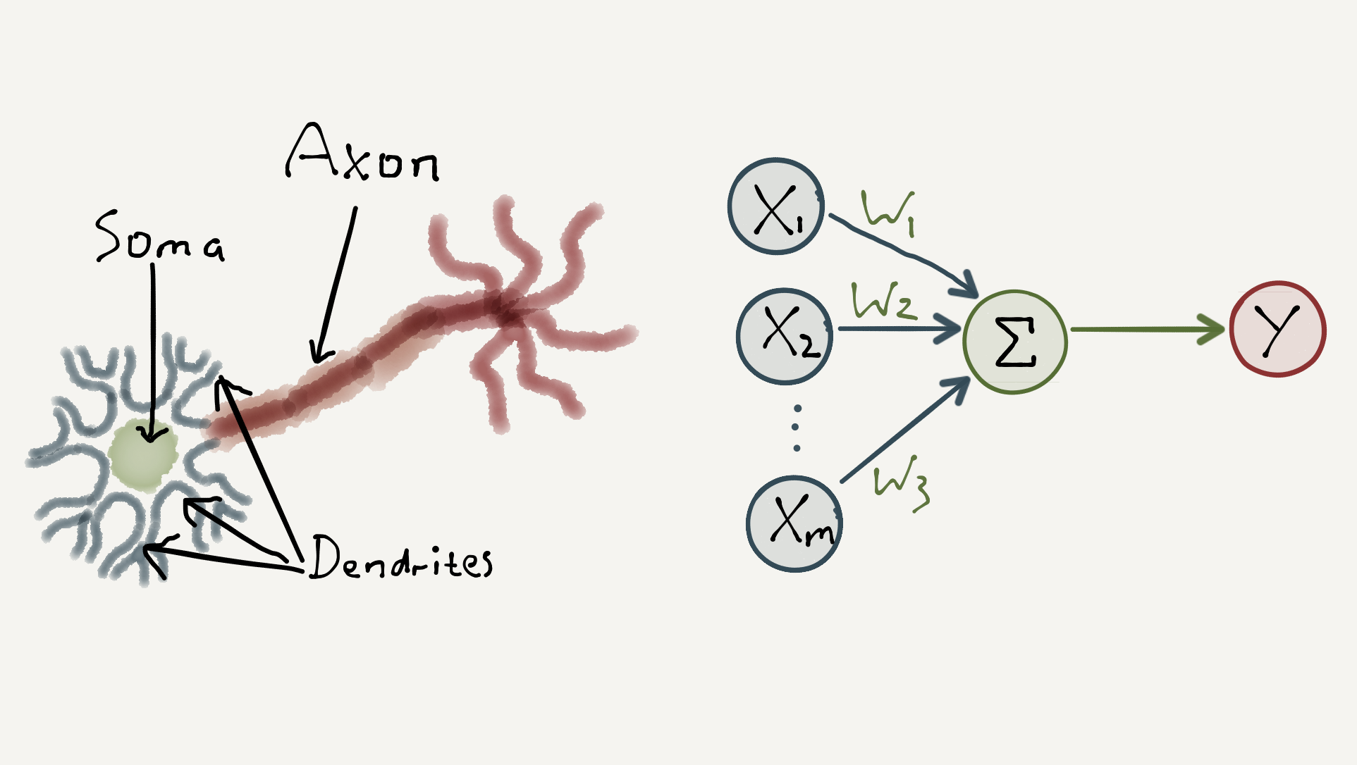
The MCP Neuron modelled this dynamic by summing a vector of input signals, \([x_1, x_2, … , x_m]\) with values \(1\) or \(0\), together with a vector of corresponding weights, \([w_1, w_2, … , w_m]\) with values \(1\),\(-1\) or \(0\). If the weighted sum of the signals exceeded some threshold value, \(t\), the model outputs a positive signal, otherwise it outputs a null signal. I.e.
\[ y = \begin{cases} 1, & \text{if} \ \sum_{i=1}^{m}w_{i}x_{i} \ \geq \ t, \\ 0, & \text{otherwise} \end{cases} \]
As an example, to model the AND gate for two input signals, we set the weights to \([1,1]\) and the threshold value to \(2\) so that all input signals must be \(1\) for the neuron to fire a positive output.
However, the problem with the MCP Neuron is that the weights had to be pre-programmed for each logic gate. Furthermore, its limited use of integers restricted the model to basic logic gates. This problem would be addressed in 1957, when the psychologist Frank Rosenblatt extended the MCP Neuron to include a learning algorithm which could automatically figure out the correct weights. He called this model the Perceptron.
Learning Algorithms: A Brief Primer
The Perceptron is an example of a supervised learning algorithm. But before we look at the Perceptron, what is a learning algorithm, and what does it mean for a learning algorithm to be supervised?
A learning algorithm is, roughly speaking, a method which adapts its computation units (for example weights in a sum) in order to achieve a desired behaviour. This is known as training.
Typically, learning algorithms are presented with examples of input data, with their correct output data, during training. This is known as supervised learning.
The class of learning algorithms that the Perceptron belongs to is known as a binary classifier. Binary classifiers learn to group data into one of two classes, typically referred to as the positive class and the negative class. In the supervised learning setting, input data used during training is already labelled as positive (\(1\)), or negative (\(-1\)). During training, binary classifiers learn a decision boundary which separates the data into the two classes.
Below is an example of a 1D decision boundary (the simplest case) on the left, and a 2D decision boundary on the right.
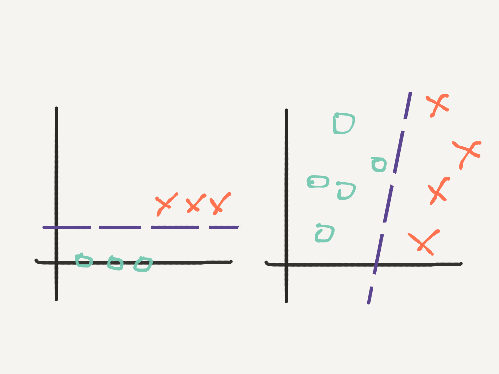
Linear decision boundaries like the examples above can be parametrised by a vector of weights, just like those in the MCP Neuron. But how does a learning algorithm figure out the correct vector of weights to fit the decision boundary?
The basic idea is illustrated below:
- Initialise the weights either to 0 or small random numbers.
- For each training example, \(x_n\), compute the predicted class, \(\hat{y_n}\), using the weighted sum: \[ \hat{y_n} = \begin{cases} 1, & \ \mathbf{w}^{T}\mathbf{x}_{n} \ \geq \ 0, \\ -1, & \ \text{otherwise} \end{cases} \]
- If a training example is misclassified, adjust the weights a little.
- Repeat 2 - 3, until the number of misclassifications is reduced to a minimum.
Note the notation from linear algebra: \(\mathbf{w} = [w_1, w_2, … , w_m]\), \(\mathbf{x} = [x_1, x_2, … , x_m]\), and \(\mathbf{w}^{T}\mathbf{x} = \sum_{i=1}^{m}w_{i}x_{i}\).
We will now make this more concrete by looking at the Perceptron learning algorithm.
The Perceptron
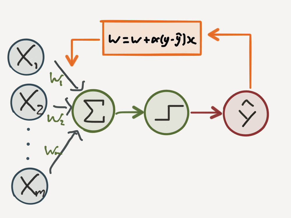
The Perceptron algorithm works by comparing the true label, \(y_n\), with the predicted label, \(\hat{y_n}\), for every training example, and then updating the weights according to whether or not the weights are too small or too large.
How do we measure this comparison? Since the labels are either \(1\) or \(-1\), one intuitive way is to note that the difference of the predicted label and the true label is \(0\) when the label is predicted correctly, and \(\pm2\), when the label is predicted incorrectly:
\[ y_{n} - \hat{y_n} = \begin{cases} 0 &, \ y_n \ = \ \hat{y_n}, \\ 2 &, \ y_n \ = 1, \ \hat{y_n} = -1, \\ -2 &, \ y_n \ = -1, \ \hat{y_n} = 1 \end{cases} \]
Since the value for \(\hat{y_n}\), depends on how large (positive) or small (negative) the weights vector is, we need to reduce \(\mathbf{w}\) when it is too large and increase it when it is too small. Using the cases above, this motivates the update rule:
\[ \mathbf{w} = \mathbf{w} + \alpha(y_n - \hat{y_n})\mathbf{x_n}
\]
There are three important factors in this update rule:
- The parameter, \(\alpha > 0\), is called the learning rate, which as the name suggests can be used to tune how quickly or slowly \(\mathbf{w}\) is updated.
- The difference \((y_n - \hat{y_n})\) will increase the weights by a factor of \(2\) when we misclassify a positive example, and decrease the weights by a factor of \(-2\) when we misclassify a negative example.
- Finally, notice that the weight update is proportional on the value of \(\mathbf{x_n}\), which ensures that we move the decision boundary to a lesser degree when \(\mathbf{w}^{T}\mathbf{x}\) is closer to zero.
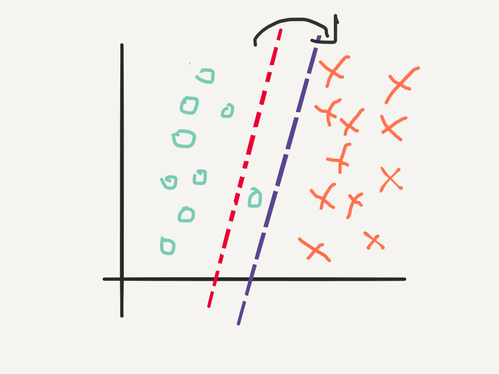
For a visual explanation of why the update rule works, consider the simple 2D case given below, with initial weights vector \(\mathbf{w} = [1, 1]\) and learning rate \(\alpha = 0.2\), and only one misclassified example.
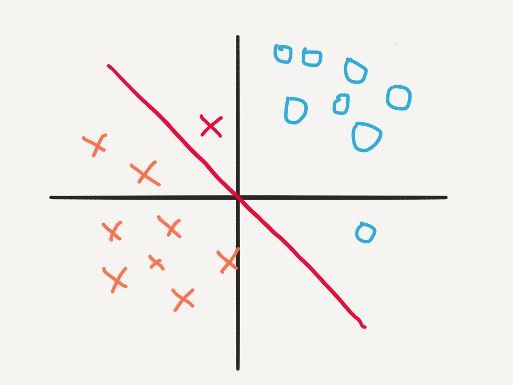
In this scenario, the training example, \(\mathbf{x^* } = [-1, 2]\), \(y^* = -1\), lies on the wrong side of the decision boundary , and indeed, \(\mathbf{w}^{T}\mathbf{x}^* = 1 > 0\), so \(\hat{y^*} = 1\). Then the update is:
\[\begin{align} \mathbf{w} & = \mathbf{w} - \alpha\big(y^* - \hat{y^* }\big)\mathbf{x}^* \\ & = \begin{bmatrix}1 \\ 1\end{bmatrix} - 0.2\big(-2\big)\begin{bmatrix}-1 \\ 2\end{bmatrix} \\ & = \begin{bmatrix}1,4 \\ 0,2\end{bmatrix} \end{align}\]
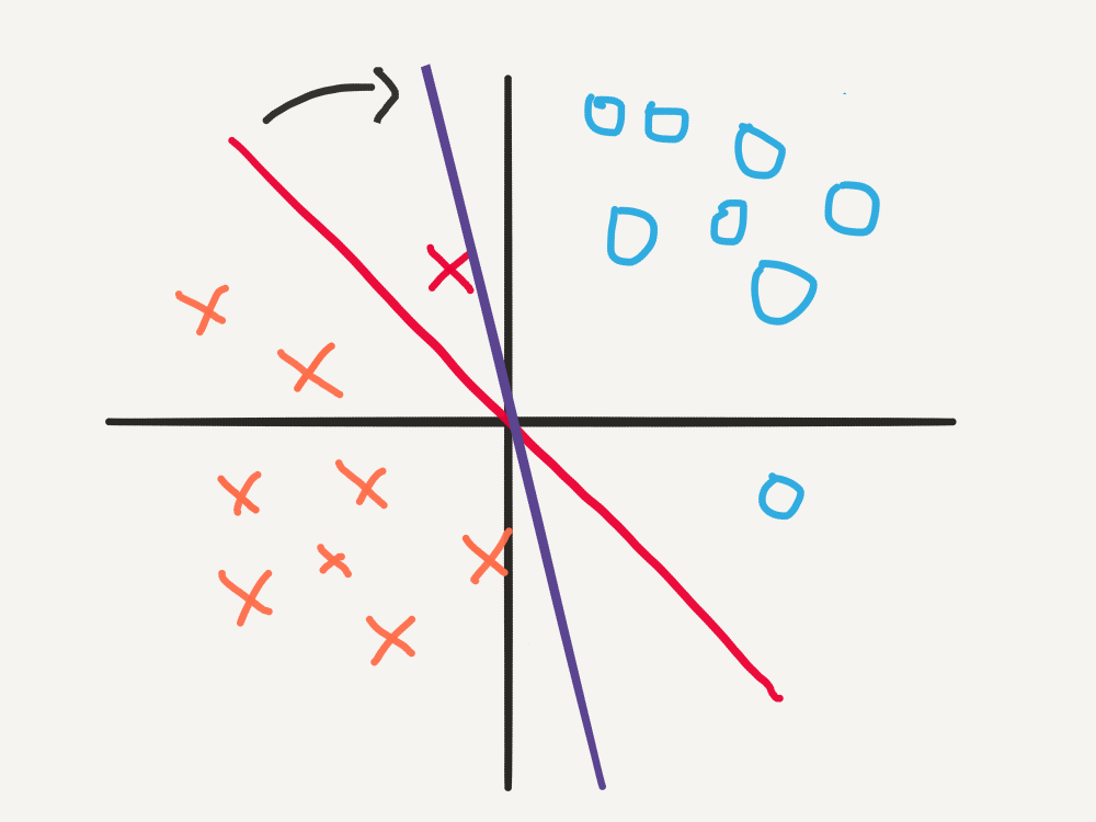
With the new decision boundary, \(\mathbf{w}^{T}\mathbf{x}^* = -1 < 0\), so \(\hat{y^*} = -1\), as required.
The Learning Rate
In the example above, the learning rate \(\alpha = 0.2\) was chosen so that the Perceptron correctly classified \(\mathbf{x^* }\) after just one update. To get an understanding of how this parameter affects convergence of the learning algorithm, we can look at what happens when we choose other values for the learning rate:
- If we set \(\alpha = 0.05\), then the updated weights vector would be \([1.1 ,0.8]\). The decision boundary is only rotated by a small amount, and thus the point \(\mathbf{x^* } = [-1,2]\) is still misclassified.
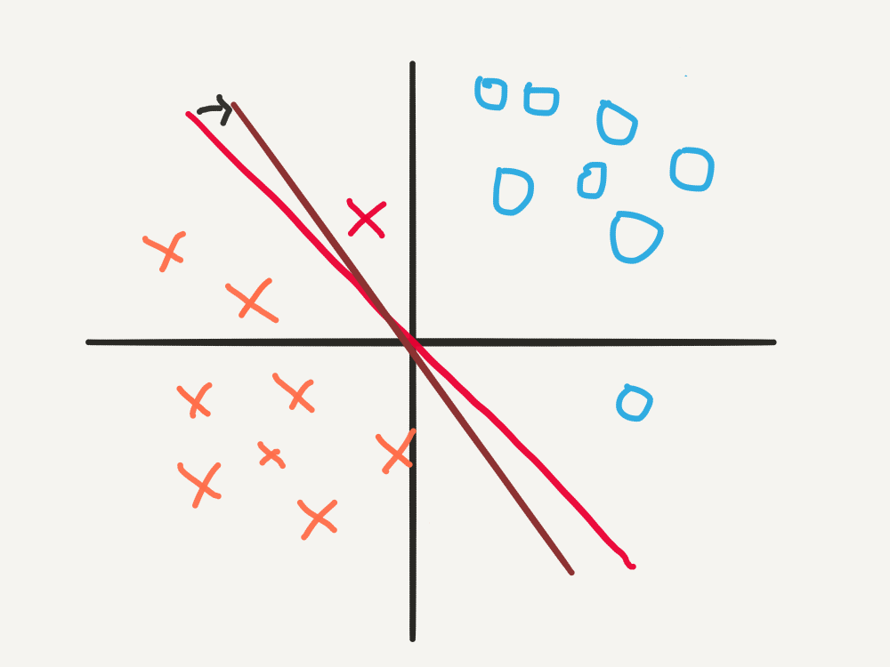
- If we set \(\alpha = 0,5\), the updated weights vector is now \([2,-1]\). The decision boundary has rotated by such a large amount, that although it correctly classifies \(\mathbf{x^* }\), it incorrectly classifies other points.
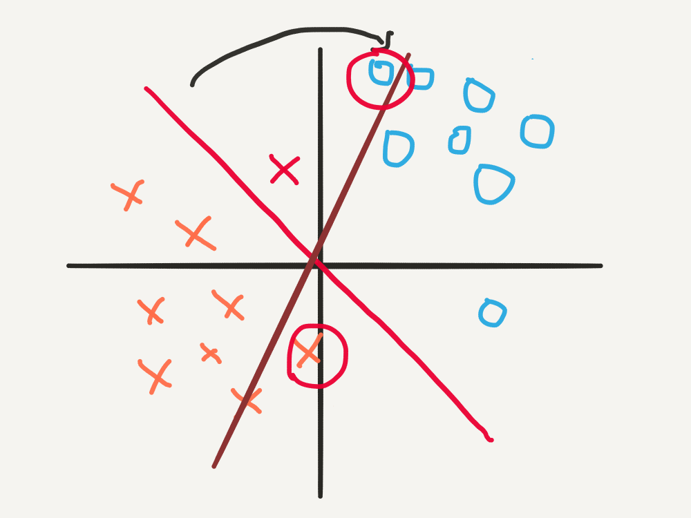
In summary, if the learning rate is too small, the learning algorithm may fail to converge in a reasonable amount of time. If the learning rate is too large, the learning algorithm may fail to settle on a good decision boundary at all! Thus we can see that the learning rate, \(\alpha\), is an important parameter in the learning algorithm, and is vital to the success of the Perceptron.
Conclusion
Introduced in 1957, the Perceptron introduced an important innovation to the field of artificial intelligence: learning algorithms. The basic premise of the Perceptron’s learning algorithm is as follows:
- If a point is classified correctly, do nothing.
- If a point is misclassified, adjust the Perceptron’s decision boundary until the point is classified correctly.
- Do this for all points, until settling on a decision boundary which minimises the number of misclassified points, possibly zero of them.
However, the Perceptron suffered from two things:
- It could only fit simple, linear decision boundaries.
- Its learning capabilities were notoriously oversold by Rosenblatt, with the New York Times reporting that it was
“the embryo of an electronic computer that [the Navy] expects will be able to walk, talk, see, write, reproduce itself and be conscious of its existence.”
The first weakness (at least) meant that it wasn’t long before the Perceptron was shown to be incapable of recognising simple non-linear patterns. Ultimately the Perceptron met its demise at the hands of the revered computer scientists Marvin Minksy and Seymour Papert in their infamous book, titled Perceptrons and released in 1969. It is believed that the criticism of Perceptrons in this book, and their extension to neural networks (explored in the next post) contributed to the so-called AI Winter - a period of reduced funding and activity in artificial intelligence researched that spanned the 1970’s, 1980’s and 1990’s.
However, as we shall explore in the next post, artificial intelligence was far from doomed, as during this period a small group of “rebel” scientists continued to work on a new type of classifier: the artificial neural network.
Special thanks go to Sebastian Raschka and Andrey Kurenkov for the inspiration, and to Andrew Ng for his passion and dedication to the field of Deep Learning. The style of this blogpost is intended to be conversational and informal. For a more formal treatment of the mathematics and code, checkout the Jupyter notebook version on Github here.
Photo by Len dela Cruz on Unsplash