The MCP Neuron

Artificial intelligence is an incredibly exciting area of research and development which spans mathematics, statistics, computer science, engineering, philosophy, linguistics, information theory, biology, pyschology, neuroscience and others. It is also a fairly nascent area of science - what has been achieved so far are just the first steps in the journey to achieving general artificial intelligence.

The success, however, of deep learning in image recognition, natural language and games, has inspired the world to take note of artificial intelligence. This success has fueled a wave of media hype and attention, that has perhaps misinterpreted what AI is for what it isn’t. AI as we know it today is not capable of thought, has no consciousness and certainly does not have any sort of intelligence that can surpass our own. Rather, the “AI” that we experience in our mobile phones, the internet or read about in the news, is a collection of computational and statistical techniques known as deep learning (or machine learning, depending on the scope).

So what is deep learning? For the best explanation of deep learning and it’s limits, I recommend this excellent two-part post by Francois Chollet, the creator of Keras. In summary, deep learning is a sequence of geometric transformations (linear and non-linear), that when applied to data, may be able to statistically model the relationships contained in that data. These geometric transformations are organised in a layered network, known as a neural network. This series is about these so called artificial neural networks, in which I will attempt to uncover what they are, how they work, where they come and why they are called “neural networks”.

Before there were any artificial neural networks, or even the perceptron (more on both in upcoming posts!), there was the MCP Neuron. First proposed in 1943 by the neurophysiologist Walter S. McCulloch and the logician Walter Pitts, the McCulloch-Pitts (MCP) neuron is a simple mathematical model of a biological neuron.

To understand how this model works, let’s begin with a very simplified (and certainly non-expert) explanation of a biological neuron. These are electrically excitable, interconnected nerve cells in the brain which process and transmit information through electrical and chemical signals. These neurons are all connected with each other to form a neural network in the brain. The connections between neurons are known as synapses. Now a single neuron in this simplified explanation consists of three parts:

Soma: this is the main part of the neuron which processes signals.
Dendrites: these are branch-like shapes which receive signals from other neurons.
Axon: this a single nerve which sends signals to other neurons.

The picture looks something like this:

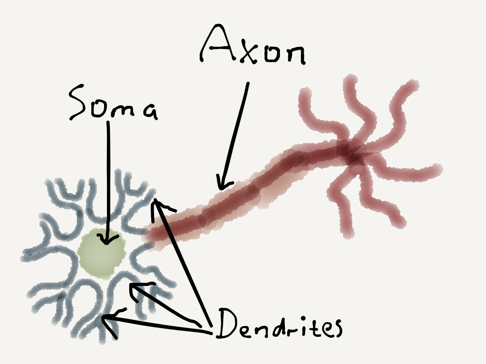
At its most basic, a single biological neuron may receive multiple signals from other neurons via its dendrites. These signals are then combined in the soma, and this combination may fire off another signal from the neuron to other neurons, which is propagated via the axon.

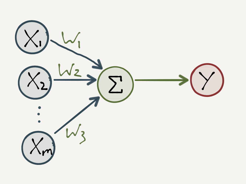
The idea behind the MCP neuron is to abstract the biological neuron described above into a simple mathematical model. The neuron receives incoming signals as \(1\)’s and \(0\)’s, takes a weighted sum of these signals and outputs a \(1\) if the weighted sum is at least some threshold value or a \(0\) otherwise. Formally this mathematical model can be specified as follows:

Let \([x_1, x_2, … , x_m]\) be a vector of input signals where each \(x_i\) has a value of \(1\) or \(0\).

Let \([w_1, w_2, … , w_m]\) be a vector of weights corresponding to the input signals where each \(w_i\) has a value of \(1\), \(-1\) or \(0\).

Input signals with a weight of \(1\) are called excitatory since they contribute towards a positive output signal in the sum.

Input signals with a weight of \(-1\) are called inhibitory since they repress a positive output signal in the sum.

Input signals with a weight of \(0\) do not contribute at all to the neuron.

Then for some threshold value \(t\), an integer, the output signal is determined by the following activation function:

\[ y = \begin{cases} 1, & \text{if} \ \sum_{i=1}^{m}w_{i}x_{i} \ \geq \ t, \\ 0, & \text{otherwise} \end{cases} \]

The neuron is said to be “activated” when the weighted sum is greater than the threshold value.

The MCP Neuron is illustrated below. Note that the \(x_i\) input signals are analogous to the dendrites, the activation function is analogous to the soma and the output is analogous to the axon.

McCulloch’s and Pitt’s original experiment was to see if they could use this model to construct different logic gates by simply specifying what the weights and threshold should be. In the next section, we’ll go through the basic logic gates and show how the MCP neuron can model them. For a corresponding Python implementation of these examples in action, checkout the corresponding Jupyter notebook on Github here.

The OR Gate

The first logic gate that we will go through is the OR gate. The OR gate indicates if there are any positive (as opposed to null) signals amongst the inputs. It will output a \(1\) if at least one of the input signals is a \(1\). For two input signals, the OR gate’s truth table looks like this:

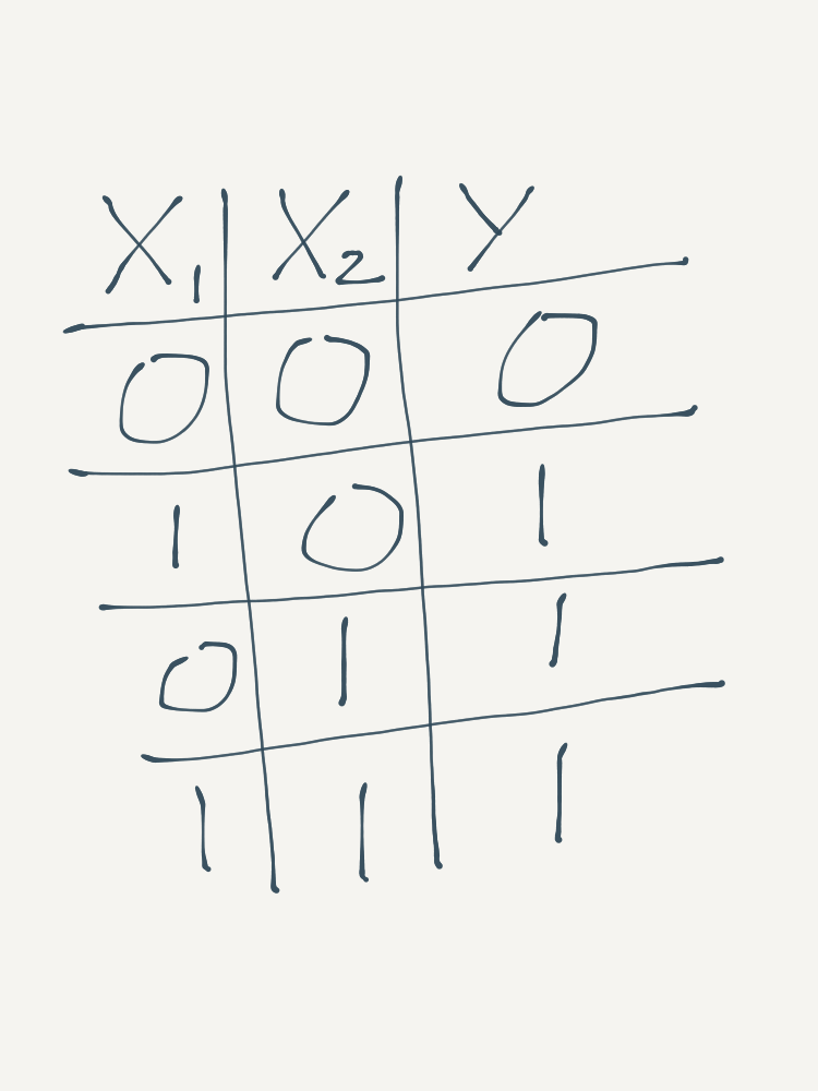
To reproduce the OR Gate using an MCP neuron, all of the weights should be \(1\), so that the neuron “considers” all inputs, and the threshold value should be \(1\), so that only one positive signal is required (at minimum) for the neuron to “activate”.

The AND Gate

The next logic gate is the AND gate. The AND gate indicates if all of the inputs signals are positive. It will output \(1\) only if all of its input signals are \(1\). It’s truth table looks this:

To reproduce the AND Gate using an MCP neuron, all of the weights should be \(1\), again so that the neuron considers all inputs, but the threshold value should be equal to the number of inputs (eg. \(2\) for the example above), so that the neuron is activated only when all inputs are positive.

The NOT Gate

So far we have seen logic gates which consider all inputs - i.e. their MCP neuron weights were all \(1\). What about gates which ignore their inputs? This can be done using a NOT gate, which inverts the signal of its input, so that if the input is positive then the output will be null and vice-versa. In short, it negates its input signal. It’s truth table is shown below:

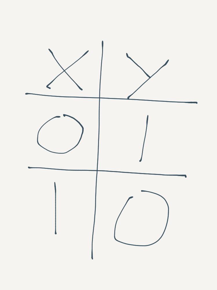
To specify a NOT Gate using an MCP neuron, set the input weights to \(-1\) and the threshold value to 0, so that the output is only ever positive when the input signal is null.

Conclusion

The MCP Neuron seems almost too simple to represent artificial intelligence of any kind, yet it is - and it isn’t. Formal logic is a fundamental component of intelligence. For any machine to have artificial intelligence, it surely should be able to comprehend logic gates. The idea being that logic gates can be stringed together to form logic circuits, capable of executing any kind of instruction. This is indeed what underpins modern computational processors. However, we know that CPU’s aren’t really “intelligent” - they’re just able to process any instruction given to them at lightning speed.

What makes the MCP Neuron different is the fact that it could reproduce logic gates using a biologically inspired algorithm. In the field of artificial intelligence, this was a promising achievement, since it almost surely makes sense that any kind of artificial intelligence should resemble the brain - which is after all the great stage of human intelligence.

The problem with the MCP Neuron is that every logic gate which it could model (and hence every logic circuit which a collection of neurons could model) had to be pre-programmed, something which is clear in the Jupyter notebook accompanying this post. This stands out as a massive contrast to the brain, which learns from experience. Nonetheless, it would take another 14 years before Frank Rosenblatt’s landmark debut of the Perceptron - the first learning algorithm of its kind. That the perceptron - and hence artificial neural networks - is a direct extension of the MCP Neuron, is what makes the MCP Neuron a cornerstone of artificial intelligence, and thus the beginning of our journey.

This is the first post in a series dedicated to the history of Artificial Neural Networks. Special thanks go to Sebastian Raschka and Andrey Kurenkov for the inspiration, and to Andrew Ng for his passion and dedication to the field of Deep Learning. The style of this blogpost is intended to be conversational and informal. For a more formal treatment of the mathematics and code, checkout the Jupyter notebook version on Github here.

Photo by Meddy Huduti on Unsplash.