In this blogpost I explore how ODE’s can be used to solve data modelling problems. I take a deep dive into the data modelling problem at hand and present ODE’s (which model rates of change) as an alternative to regression (which attempts to model data directly). Later I introduce the extension to neural ODE’s. To keep the focus on neural ODE’s I’ll assume that you have knowledge of linear regression, deep learning and basic calculus.
This is a long post and I hope that you will take the time to read it in its entirety. I’ve split the post into 5 numbered parts, which I summarise at the end as 5 conceptual steps (leaps). If at times you feel that you are losing track of the bigger picture, then feel free to scroll to the end to see where each idea fits.
Many of you may have recently come across the concept of “Neural Ordinary Differential Equations”, or just “Neural ODE’s” for short. Based on a 2018 paper by Ricky Tian Qi Chen, Yulia Rubanova, Jesse Bettenourt and David Duvenaud from the University of Toronto, neural ODE’s became prominent after being named one of the best student papers at NeurIPS 2018 in Montreal. Shortly afterwards a media feature in the MIT Tech Review and a front page appearance on Hacker News helped propel neural ODE’s into the machine learning limelight.
MIT Tech Review described the architechture as a “radical new design” with the “potential to shake up the field—in the same way that Ian Goodfellow did when he published his paper on GANs.”
This may sound like hype, and perhaps it is, however I’m intrigued and excited by neural ODE’s for several reasons. At first glance they appear to have immediate practical advantages (this is where I believe the hype differs from GANs), for example in continuous time settings. Secondly ODE’s have a long history in applied and pure mathematics. They are well studied in physics, engineering and other sciences. Most modern scientific programmes have extremely well-tested and high performing differential equation libraries.
Finally neural ODE’s bring a powerful modelling tool out of the woodwork. When I was an undergrad in mathematics, we were taught that we solve applied maths problems using differential equations. Today we are taught that we solve applied maths problems using machine learning. I got into machine learning because I found neural networks to be the most promising tool for solving problems with maths. Neural ODE’s open up a different arena for solving problems using the muscle power of neural networks.
In a word, they are a indeed a “radical” new paradigm in machine learning.
In this blogpost I explore this new paradigm, starting with the initial data modelling problem. I’ll introduce ODE’s as an alternative approach to regression and explain why they may hold an advantage. I’ll give a brief perspective of the world of numerical ODE solvers. After that I’ll introduce neural ODE’s as they are described in the paper. I’ll briefly explain how backpropogation is implemented, which is the major contribution of the paper. Finally I will bring everything together.
1. Modelling Data
In a classical data modelling setting we have a set of \(N\) pairs of data points, \(\mathscr{D} = \big\{(x_1, y_1), (x_2, y_2), …, (x_N, y_N)\big\}\). \(\mathscr{X}\) is the input domain and \(\mathscr{Y}\) is the output domain. Given a new data point, \(x^{*}\), we would like to make a prediction about it’s value \(y^{*}\). We can view this problem as:
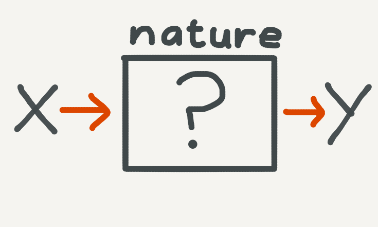
Nature generates the data: we can try and describe the data using an algorithm and then use the resulting model to make new predictions. For more on this approach, see the seminal essay, Two Cultures, on data modelling by the late Leo Breiman.
Our original dataset is generated by nature (physical, social, economic or otherwise). We have no good sophisticated way of remodelling a reliable data generation process, so instead we treat nature as a black box and bypass it with an algorithm. The machine learning approach is to iteratively find a function which best describes the data. The process of finding this function is known as a learning algorithm. In short, machine learning can be thought of as repurposing the original data modelling problem into a function approximation problem. In modern machine learning, particularly deep learning, these functions are highly flexible neural networks. Thus the original data modelling problem becomes something like this:
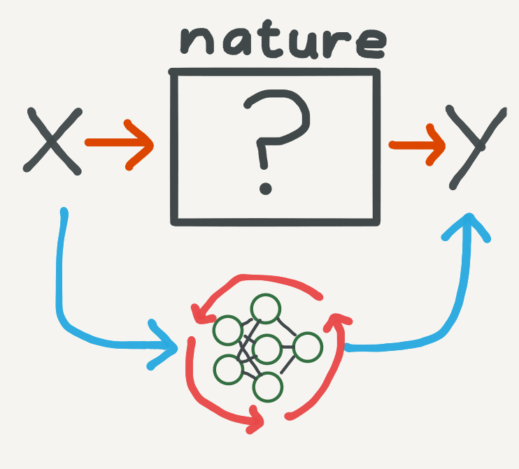
Neural networks can be viewed as an algorithmic approximation which bypasses the generative process of the data. They are trained over many iterations of an optimisation loop.
Part of the success of machine learning (which I will use interchangeably with deep learning) lies in the enormous flexibility of neural networks. They are high-dimensional, have millions of parameters over which we can compress patterns found in data, are highly nonlinear and can be implemented using highly optimised computing frameworks.
However, in order to understand where neural ODE’s fit in, it will be useful to abstract away from neural networks and return to the original function approximation perspective.
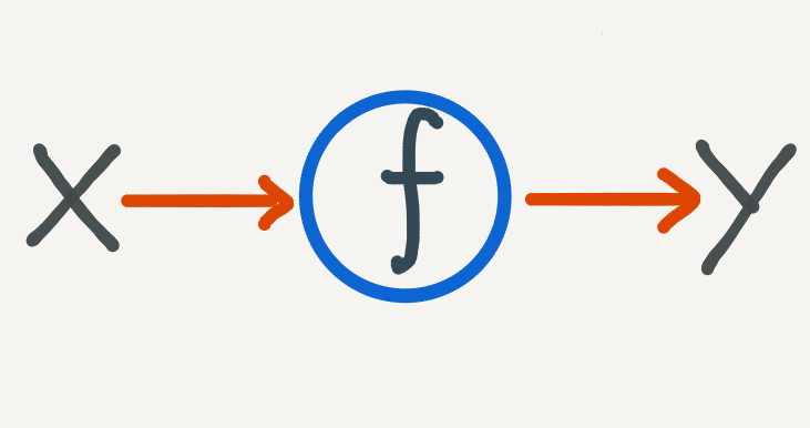
Our ultimate goal will be to find a robust mapping from \(\mathscr{X}\) to \(\mathscr{Y}\).
We are now at the fundamental mathematical problem where there is some function, which we would like to know, which sends points in \(\mathscr{X}\) to points in \(\mathscr{Y}\):
\[
f: \mathscr{X} \to \mathscr{Y}.
\]
Two Basic Approches: ODE’s vs Regression
Given the dataset, \(\mathscr{D}\), there are two basic approaches for solving this problem. The first approach, known as regression, should be familiar to anyone working in machine learning. The other approach, which is the dark horse here, is to use an ordinary differential equation.
To explain these two approaches, let’s suppose that \(\mathscr{X}\) and \(\mathscr{Y}\) are both just the ordinary real number line, \(\mathbb{R}\), so that the problem can be visualised and intuitioned easily, and that we have the following arbitrary data points:
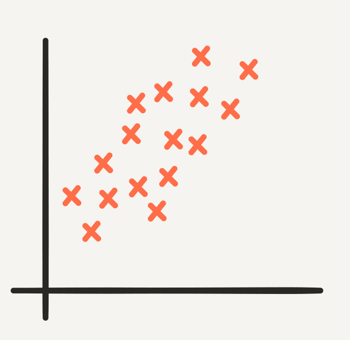
Linear data in \(\mathbb{R}^2\).
How should we go about finding the function
\[
f: \mathbb{R} \to \mathbb{R}.
\]
which best describes the data?
Curve Fitting
I’ve kept this situation simple and low dimensional so that we can use ordinary linear regression. The data has a somewhat linear shape so we describe it using the parametric form of a line:
\[ \widehat{y} = ax + b, \]
where \(y_i = \widehat y_i + \epsilon\), and \(\epsilon\) is an error term added to our model, representing random noise in the data. In linear regression we try to minimise the mean square error
\[ \mathscr{L}(a, b) = \frac{1}{n}\sum_{i=1}^{N}\big(y_i - \widehat{y}_i\big)^2. \]
The mean square error is a loss function which is a function of the parameters \(a\) and \(b\) - since we take our data as fixed and each \(\widehat y_i\) is evaluated at known \(x_i\) for unknown \(a\), \(b\). In machine learning we find the optimal choice of the parameters which minimise the loss function. Call them \(a^*\) and \(b^*\). The function which we’ve approximated is then the line
\[ f^*(x) = a^*x + b^*, \]
which will look something like this:
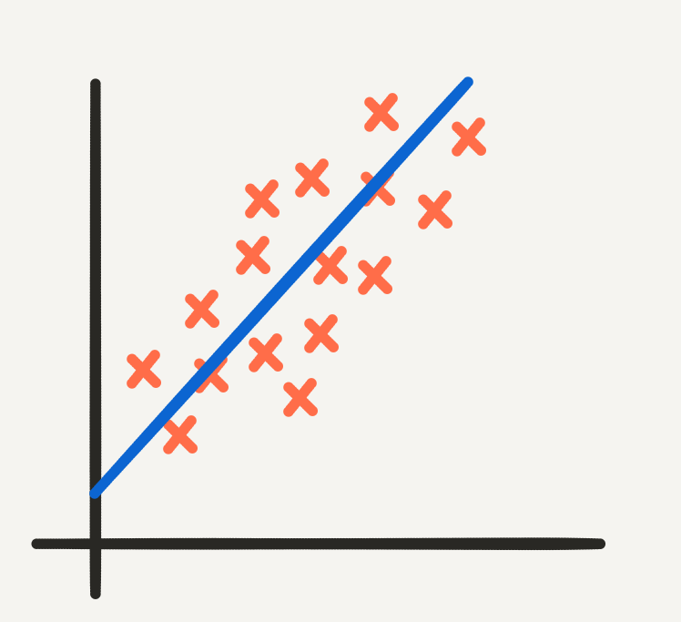
The line of best fit produced by linear regression.
In general this is known as curve fitting.
2. Modelling Rates of Change
In order to optimise the loss function we typically require the function which we’re approximating to be differentiable. In research and in practice, great care is taken to ensure that neural network architectures are indeed differentiable. Now in Calculus I, we learn that every differentiable function \(f\) has a derivative \(f’\), which is the continuous limit of the rate of change of \(f\):
\[ \frac{df}{dx} = f’. \]
We also learn in calculus that if a function satisfies certain continuity properties then we can go the other way round and integrate it, so that if
\[ F(x) = \int f(x)dx, \]
then
\[ F’(x) = f. \]
How does this relate to our modelling problem? With regression, we assumed that there was a continuous and differentiable relationship between \(x\) and \(y\), described by the function \(f\):
\[ y = f(x). \]
In regression we try to find \(f\) directly. But if \(f\) is differentiable, what if we tried to find its derivative instead? This amounts to searching for \(f\) indirectly by differentiating the regression relationship:
\[ \frac{dy}{dx} = f’(x). \]
This is a basic form of an ordinary differential equation, or an ODE. Solving the ODE is equivalent to solving the integral
\[ f(x) = \int f’(x)dx, \]
and can therefore be viewed as function approximation, only here we are approximating the derivative instead.
ODE’s: Basic Form
In the basic form of an ODE we allow the derivative to depend not only on \(x\), but also on \(y\). This allows for greater modelling flexibility. Now in calculus you learnt that the integral depends on at least one unknown constant value. To solve for this constant we need a pair of points, \(x_0\) and \(y_0\). If there is more than one constant, we need more pairs of points. Luckily in the machine learning scenario we have an entire dataset, \(\mathscr{D}\), of \(N\) data points!
The functional form of the integral will depend on the approximating function we choose for the derivative. The precise form of the integral will depend on the data.
To keep the notation limited, we’ll use \(f\) to denote the function describing the derivative in the ODE. The setup is then,
\[ y’(x) = f(x, y), \ \ \ \ y(x_0) = y_0, \]
where \(y(x)\) is interpreted as “the value of \(y\) at \(x\). From the most abstract point of view, nothing much has changed. We are still interested in finding some function - called \(f\). What has changed fundamentally, however, is that now this function describes the rate of change - how \(y\) changes as \(x\) changes - as opposed to the direct relationship.
Why is this useful? We’ll see that approximating derivatives reduces the number of parameters, and also the number of function evaluations (computal cost) required to find the optimal parameters.
Parametric Efficiency
Let’s go back to the dataset I showed earlier in \(R^2\). In the regression scenario, we made the assumption that the function we are trying to approximate is linear, i.e.
\[ y \approx f(x) = ax + b. \]
In this case there are two free parameters, \(a\) and \(b\).
The term free means that these parameters are allowed to vary as we try to minimise the loss. They are the parameters which we are interested in optimising.
What if we used the ODE approach instead? We know the parametric form of the derivative, which we can write as:
\[ \frac{d\widehat y}{dx} = a. \]
Now we are trying to approximate the function:
\[ \frac{dy}{dx} \approx f(x, y) = a. \]
Immediately we can see that there is only one free parameter, \(a\).
If we were to solve this problem analytically, we would still end up needing to solve for the parameter \(b\). However most interesting ODE problems can’t be solved analytically and require numerical methods.
These numerical methods are implicit in that they don’t analytically give you the integral but rather a set of function evaluations at future points. Thus we don’t need to care about the extra parameter \(b\) at all. All we need is an initial point \((x_0, y_0)\) to get us started and any number of additional points from our data to tune the fit.
It turns out that optimising an ODE can be more computationally efficient than regression. In order to explain this, it will be helpful to look a bit more into numerical integration.
Numerical Methods for ODE’s
When we can’t find the solution to an ODE analytically, and this is often the case in practical situations, we need to resort to numerical methods which approximate a solution at discrete evaluation points.
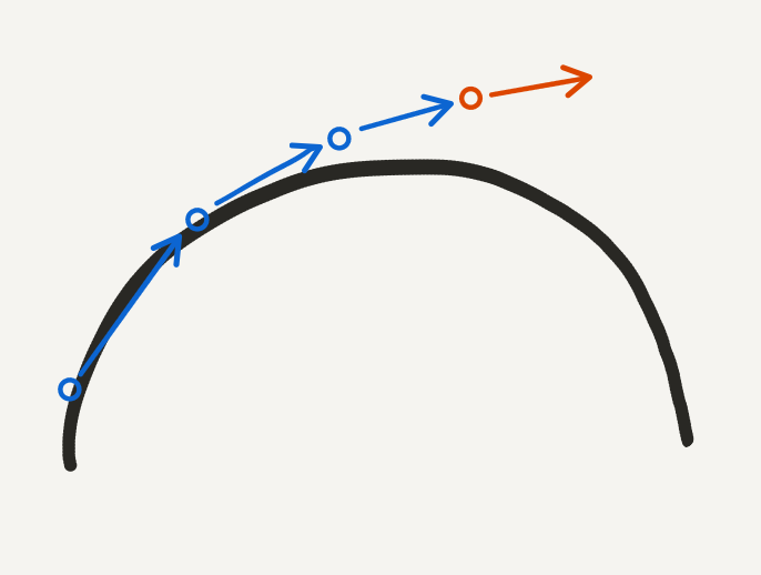
How do we go about finding the solution to an ODE numerically? For starters the gradient of the integral we are trying to solve is available to us - in our setup it is \(f(x,y)\) - and we know that the gradient traces the curvature of the function we’re trying to solve for. The picture below describes this for the parabola:
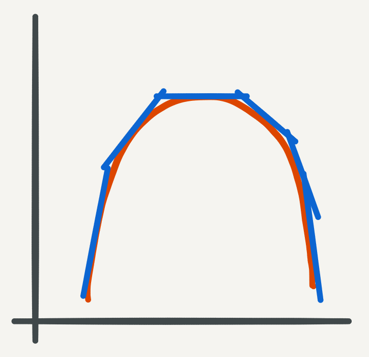
Gradients tracing the parabola.
So we can use precisely this logic to compute integrals numerically. We can start at an initial point and move in the direction of the gradient evaluated at the initial point to get to a new evaluation point. Starting at this second evaluation point we can repeat the same procedure to move on to a third evaluation point, and so on.
This is the basic idea behind Euler’s method. While it seems simple, Euler’s method is a starting point for advanced numerical methods, which build on this basic idea with more sophisticated updates at each step. Typically a single step will be composed of smaller steps, sometimes using higher order gradients where available. The more substeps that are taken, the higher the fidelity of the method.
Euler’s method falls in to two larger classes of methods: Runge-Kutte methods and Adams-Bashforth methods. In both cases, Euler’s method is the simplest order method.
Euler’s Method
To describe Euler’s method, we’ll replace the symbol for the input domain by \(t\). By convention we’ll interpret \(t\) as being a time element in the evolution of \(y\) as we iteratively use the method. This will also tie in better with the paper. Euler’s method is derived from the basic definition of the tangential approximation of the gradient at a point:
\[ \frac{dy}{dt} \approx \frac{y(t + \delta) - y(t)}{\delta}, \]
where \(\delta\) is a fixed step-size. We can rearrange this expression to get:
\[ y(t + \delta) = y(t) + \delta\frac{dy}{dt}. \]
This is an explicit algebraic description of the stepwise procedure which I described and illustrated above. We can then plug in the functional formula for the derivative to get
\[ y(t + \delta) = y(t) + \delta f(t, y). \]
Finally to compute approximations for \(y\) using Euler’s method, we need to discretize the domains. Starting from an initial point \((t_0, y_0)\), we define a computation trajectory recursively as follows:
\[ t_{n+1} = t_{n} + \delta (n+1), \ \ \ \ n = 0, 1, 2, … \] \[ y_{n+1} = y_{n} + \delta f(t_{n}, y_{n}), \ \ \ \ n = 0, 1, 2, … \]
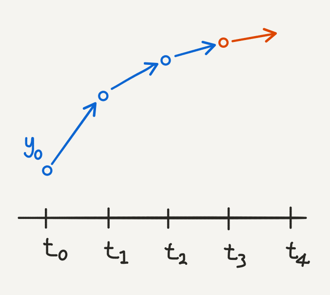
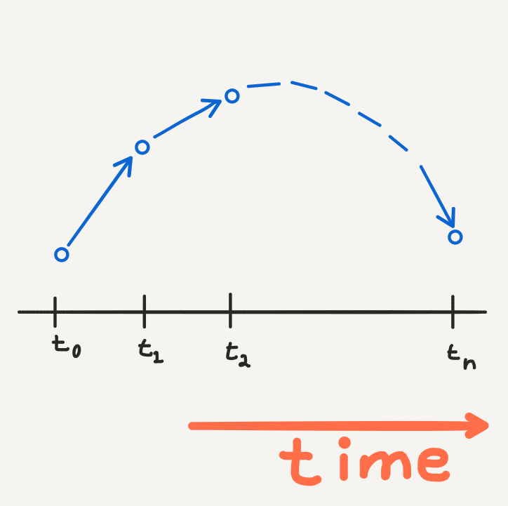
Euler’s method illustrated: at each time point, we use the current value of \(y\) to calculate the next value. The gradient tells us which direction to move in and by how much.
Optimising the ODE
At this point we have a modelling assumption that
\[ \frac{dy}{dx} = f(x, y) = a, \]
and we have a numerical method for evaluating \(y\) at different values of \(x\). However to use Euler’s method we need to explicitly define \(f(x, y)\), which requires that we have a value for \(a\).
The machine learning paradigm is to treat a as a free parameter which we can optimise.
In particular we can make an initial guess for \(a\) and use Euler’s method to compute the forward pass on our data. Each numerical method is different, but for Euler’s method we will compute the forward pass as follows:
- Choose an initial value for \(a\) and a fixed stepsize \(\delta\)
- Choose some \((x_0, y_0)\) to be the initial value. Choose \(k\) data points to evaluate at, and order your choices. Choosing \(k < N\) points can reduce the scaling complexity of ordering.
- Add additional points from \(\mathscr{X}\) so that you can use Euler’s method at regular intervals. This is your computation trajectory.
- Compute Euler’s method along your computation trajectory, also evaluating at your chosen points from your data.
You can then calculate the loss by comparing Euler’s method evaluated at the \(k\) chosen datapoints with their actual values. In the backward pass you can calculate a derivative of your loss function with respect to \(a\), for each evaluation point, and adjust it as you would in gradient descent.
In summary, by using Euler’s method in the context of a machine learning optimisation problem, we treat \(a\) as a free parameter. Importantly \(a\) is the only free parameter and can be used to describe a linear relationship which typically requires two parameters.
Computational Cost
This process is also more compuationally efficient. In the simple linear regression example we can solve for the free parameters analytically using well known formulas. However in more complex regression (and classification) problems we use gradient descent to solve for the parameters. Each step of gradient descent requires computing the loss at every datapoint. Even if we use stochastic gradient descent, we still require several epochs, passing through the whole dataset, in order to find the optimal parameters. Throughout training we ultimately rely on not only the entire dataset itself, but also on performing function evaluations on the entire dataset during the forward and backward pass.
With an ODE, we require only one initial datapoint to get started. We can then perform \(N\) function evaluations at each point in the forward pass. We then need to only evaluate the loss function at a handful of data points, before deciding how to update the free parameters. We can run this for several epochs until we’re satisfied. Ultimately, solving for an ODE requires fewer function evaluations, particularly in the backward pass. In fact, one of the contributions made in the paper is to show that this tends to be emperically true for neural ODE’s as well.
If we use modern implementations in numerical ODE methods, then we’re in even better luck. These solvers are designed to adapt the amount of computation required so that the number of function evaluations can be decreased if it doesn’t impact error.
To get an intuition for why we do not need the whole dataset, consider a situation where we are trying to fit a parabola which requires two parameters to describe the derivative:
\[ \frac{dy}{dx} = ax + b. \]
After choosing an initial guess for \(a\) and \(b\) and an initial data point, we can run several iterations of Euler’s method and compare it to the true data:
Euler’s method diverging: simple methods like Euler’s method can easily diverge. More advanced methods will be more robust.
We only need to evaluate Euler’s method at the most recent function evaluations to determine if it is diverging. We can then use gradient descent to adjust the free parameters.
3. Neural ODE’s
So far I’ve described how we can use an ODE to solve a data modelling problem. We approximate the relationship between points in our input and output domain by optimising the functional form of the rate of change:
\[ \frac{dy}{dx} = f(x, y). \]
With deep learning we can go even further. We know that neural networks are universal function approximators. So what if we used our neural network to approximate \(f\)? In theory if we can approximate the derivative of any differentiable function using a neural network, then we have a powerful modelling tool at hand. We also have a lot more flexibility in the data modelling process.
In particular, consider a neural network where the hidden states all have the same dimension (this will also be helpful for visualising their evolutionary trajectories later). Each hidden state depends on a neural layer, \(f\), which itself depends on (free) parameters \(\theta_t\), where \(t\) is the layer depth. Then
\[ h_{t+1} = f(h_{t}, \theta_{t}). \]
If we have a residual network, then this looks like
\[ h_{t+1} = h_{t} + f(h_{t}, \theta_{t}). \]
One of the intuitions which inspired the paper is that this has a similar form to Euler’s method which we described above. To understand this, remember that Euler’s method is a discretisation of the continuous relationship between the input and output domains of the data. Neural networks are also discretisations of this continuous relationship, only the discretisation is through hidden states in a latent space. Residual neural networks create a pathway through this latent space by allowing states to depend directly on each other, just like the updates in Euler’s method.
Residual neural network appears to follow the modelling pattern of an ODE: namely that the continuous relationship is modelled at the level of the derivative.
To take this logic full circle, we consider the continuous limit of each discrete layer in the network. This is the radical idea proposed by neural ODE’s. Instead of a discrete number of layers between the input and output domains, we allow the progression of the hidden states to become continuous:
\[ \frac{dh(t)}{dt} = f(t, h(t), \theta_t), \]
where \(h(t)\) is the value of the hidden state evaluated for some \(t\), which we understand as a continuous parametrisation of layer depth. The arena is opened up for solving the data problem as a Neural ODE. The next step is to explore this dynamic even further.
4. Continuous Hidden State Dynamics
In Euler’s method we defined a computation trajectory by starting from some initial point \((t_0, y_0)\) and recursively evaluating the ODE at fixed step sizes:
Euler’s method traces an appoximate evolution of \(y\) through time.
The fixed stepsizes represent a time scale in the evolution of the ODE as we solve it numerically. This defines a dynamic of the outcome \(y\) with respect to time. In fact the functional form of the ODE neatly represents this idea:
\[ \frac{dy}{dt} = f(t, y). \]
Now the key feature of a neural network is that we add in hidden states between the input and outcome:
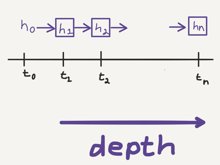
Hidden state evaluations in a neural network: we can view the transformation made by each layer as an evolution of the hidden state through time.
This looks similar to the computation trajectory of Euler’s method. Only now the fixed stepsizes correspond to the layers in the neural network, which defines a dynamic of the hidden state with respect to depth. This dynamic can be visualised as a discrete evolution of the hidden state, evaluated at each layer:
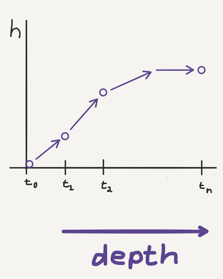
Discrete hidden state trajectory: we can plot how the hidden state evolves through each layer in a neural network.
When we take the continuous limit of the hidden state with respect to depth, we smooth out this computation trajectory so that in theory, the hidden state can be evaluated at any “depth”, which we now consider to be continuous:
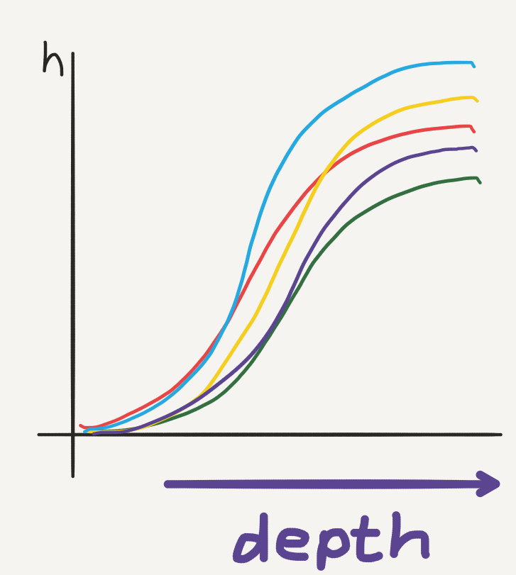
Hidden state dynamics: the continuous hiddens state trajectories will vary with the free parameters.
In a neural ODE, we parametrise this hidden state dynamic by
\[ \frac{dh(t)}{dt} = f(t, h(t), \theta_t), \]
where \(f(t, h(t), \theta_t)\) is a neural network layer parametrised by \(\theta_t\) at layer \(t\).
We can evaluate the value of the hidden state at any depth by solving the integral
\[ h(t) = \int f(t, h(t), \theta_t)dt. \]
How do we solve this integral? Using a numerical ODE method of course. The final modelling assumption is to take the input as \(h(t_0) = x\) - i.e. the initial value of the ODE - and to let the output be evaluated at some time \(t_1\), so that \(h(t_1) = y\). The function approximation problem now takes place over a continuous hidden state dynamic:
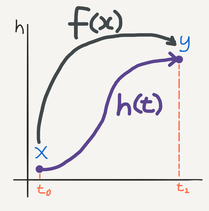
Function approximation over hidden state dynamics: ultimately we are finding an implicit mapping \(F\) going from \(\mathscr{X}\) to \(\mathscr{Y}\).
How do we decide what the values for \(t_0\) and \(t_1\) are? Well, since this is a machine learning approach we can treat them as two additional free parameters to be optimised. We can put everything together into a numerical ODE solver of our choice, which we can just call \(ODESolve\) in the spirit of the paper, so that:
\[
\widehat{y} = h(t_1) = ODESolve\big(h(t_0), t_0, t_1, \theta, f\big),
\]
where \(f\) is a neural network.
5. Backpropogating Through Depth
The central innovation of the paper is an algorithm for backpropagating (reverse-mode differentiation) through the continuous hidden state dynamics. In the neural ODE, our parameters are not just \(\theta_t\), but also the evalutation times \(t_0\) and \(t_1\). As usual we can define any (differentiable) loss function of our choice on these (free) parameters:
\[ \mathscr{L}(t_0, t_1, \theta_t) = \mathscr{L}\Big(ODESolve\big(h(t_0), t_0, t_1, \theta, f\big)\Big). \]
To optimise the loss, we require gradients with respect to the free parameters. As with the usual backpropagation algorithm for deep learning, the first step is to compute the gradient of the loss with respect to the hidden states:
\[
\frac{\partial\mathscr{L}}{\partial h(t)}.
\]
But the hidden state itself is dependent on time (depth), so we can take a derivative with respect to time. Bear in mind that this time derivative will be a reverse traversal of the hidden states, which we will need to keep track of. This is where the adjoint method comes in, which is a decades old numerical technique for efficiently computing gradients.
A proof for the adjoint method and how it is used in the paper can be found in Appendix B of the paper. For an accessible explanation of the adjoint method see this blogpost by Kevin Gibson.
To keep track of the time dynamics, we’ll define the so-called adjoint state
\[
a(t) = -\frac{\partial\mathscr{L}}{\partial h(t)}.
\]
The adjoint state represents how the loss depends on the hidden state (remember that this is continuous along a trajectory) at any time \(t\). It’s time derivative is given by the following formula:
\[ \frac{da(t)}{dt} = -a(t)^{T}\frac{\partial f(t, h(t), \theta_t)}{\partial h(t)}. \]
This derivative is computable since the loss, \(\mathscr{L}\), and \(f\), which is precisely a neural network, are both differentiable by design. This derivative also happens to be an ODE, so we can write down the solution of the adjoint state as the integral:
\[ a(t) = \int -a(t)^{T}\frac{\partial f(t, h(t), \theta_t)}{\partial h(t)} dt, \]
or equivalently
\[ \frac{\partial\mathscr{L}}{\partial h(t)} = \int a(t)^{T}\frac{\partial f(t, h(t), \theta_t)}{\partial h(t)} dt, \]
We can solve this integral by making a different call to an ODE solver. To get the gradient at \(t_0\), we can run this ODE solver backwards in time from the initial point which is known to us (just like usual backpropagation) at time \(t_1\):
\[ a(t_0) = \int_{t_1}^{t_0} -a(t)^{T}\frac{\partial f(t, h(t), \theta_t)}{\partial h(t)} dt, \]
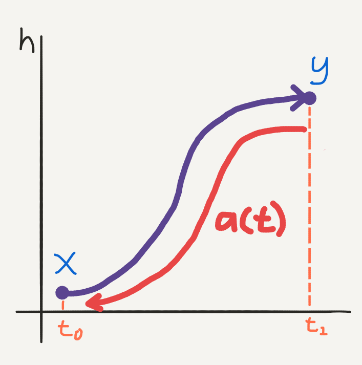
Backpropagation using the adjoint method: the adjoint state is a vector with its own time dependent dynamics, only the trajectory runs backwards in time. We can solve for the gradients at \(t_0\) using an ODE solver for the adjoint time derivative, starting at \(t_1\).
Now at this stage we have a way of computing the gradient with respect to \(t_1\) and \(t_0\). This covers two of the parameters. To compute gradients with respect to \(\theta\) we solve the ODE (also proven in Appendix B):
\[ \frac{\partial\mathscr{L}}{\partial\theta} = \int_{t_1}^{t_0} a(t)^{T}\frac{\partial f(t, h(t), \theta_t)}{\partial\theta} dt. \]
Again this integral can be solved using an ODE solver. However the paper insists that we can do even better. All three integrals can be computed using only one call to an ODE solver by vectorising the problem. This is described in Appendix B.
(Optional) Augmented State Dynamics
The rest of this section is based on Appendix B of the paper. It is more mathematically involved but worth going through to understand the computational implementation of backpropagation for neural ODE’s. Feel free to skip ahead to the final section and come back to this point at a later stage.
- Let \(\theta\) be “independent of time” such that \[ \frac{d\theta}{dt} = 0, \] and observe that \[ \frac{dt}{dt} = 1. \]
- Let \([h, \theta, t]\) represent an augmented state, then we can define the augmented state function:
- Then let the augmented state dynamics be given by:
- This is an ODE which has augmented adjoint state:
where \(a\) is the adjoint for the hidden state described above:
\[ a = -\frac{\partial\mathscr{L}}{\partial h}, \]
and \[ a_\theta = \frac{\partial\mathscr{L}}{\partial\theta}, \ a_t = \frac{\partial\mathscr{L}}{\partial t}. \]
The time derivatives of this adjoint state can then be computed using the following formula (if you know anything about vector calculus, then the details can be found in Appendix B of the paper): \[ \frac{da_{aug}}{dt} = - \biggl[ a\frac{\partial f}{dh}, \ a\frac{\partial f}{d\theta}, \ a\frac{\partial f}{dt} \biggr]. \]
The entire backpropagation algorithm can now be solved by making a call to an ODE solver on the augmented state dynamics.
Tying Everything Together
Thank you for making it to this point. I hope that you now have a better understanding of how neural ODE’s can help solve your data modelling problem.
My intention is to explain intuitively how ODE’s can model a simple modelling problem, and how they can be optimised (in a simple scenario). The second half of this post extended that simple model to the neural ODE model as it’s presented in the paper. We covered how an ODE problem can be paramatrised by a neural network and how the neural network parameters can be optimised by backpropagating through the ODE using the adjoint method.
For now, it is worth reiterating the neural ODE approach to solving a data modelling problem.
- We have a set of \(N\) pairs of data points, \(\big\{(x_1, y_1), …, (x_N, y_N)\big\}\). Given a new data point, \(x^{*}\), we would like to make a prediction about it’s value \(y^{*}\). We seek a functional approximation to the relationship between the input and output domains.
- Instead of modelling this relationship directly, we model the derivative: \[ \frac{dy}{dx} = f(x, y). \]
- We paramatrise this approximation by a neural network with hidden states \(h(t)\), depending continuously on layer depth \(t\), with \(h(t_0) = x\) and \(h(t_1) = y\). The function approximation problem is now \[ \frac{dh(t)}{dt} = f(t, h(t), \theta), \] where \(f\) is a neural network.
- This is an ODE describing continuous hidden state dynamics. We can solve the data modelling problem by solving this ODE. This reduces to solving the integral \[ h(t) = \int f(t, h(t), \theta) dt. \] To make predictions we solve the definite integral \[ \widehat{y} = h(t_1) = \int_{t_0}^{t_1} f(t, h(t), \theta) dt. \] The analytical solution of this integral is not available to us. Instead we can use a numerical method (available to us using modern numerical computation software) to solve the integral at the required evaluation points: \[ \widehat{y} = h(t_1) = ODESolve(h(t_0), t_0, t_1, \theta, f). \]
- The free parameters of this problem are \(t_0\), \(t_1\) and \(\theta\). We optimise our choice of these free parameters by backpropagating through the ODE solver using the method of adjoints.
Photo by Randall Ruiz on Unsplash